
Recent changes, updates and additions in the available Gecco exposure data
Last update: 21 March 2025
Updated by: Alfred Wagtendonk / Gecco
For explanation on spatial operations and terminology used please click here.
March 2025
Summary: New air traffic map 2022
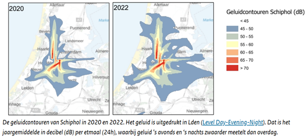
Atlas Living Environment had a map with aircraft noise from 2020. But that year, the number of flight movements was historically low due to corona. Atlas Living Environment now has data on air traffic in 2022. Air traffic has increased compared to 2020, but in 2022 there are still fewer flights than before corona.
See the news section from Atlas Leefomgeving for more details, graphs and the situation at other airports.
March 2025
Summary: Land use map 2020 from CBS soils statistic office published
After many years of waiting the CBS soil statistics office finally published this winter (November 2024) the land use map of 2020 and coming summer also the land use map of 2022 is expected. The reason for the long waiting is the application of a new production methodology for the land use maps, which has also consequences for land use comparison with earlier years. For more explanation read the technical documentation.
I will add the derived products of this new landuse map (in particular the components and the total walkability score for the year 2020) as soon as possible, probably in the course of April.
In the mean time you can find the new land use map for 2020 here:
geodata.cbs.nl - /files/Bodemgebruik/NBBG2020/
Note that some new landuse classes were added:
13 Metro en sneltram (Metro and light rail)
36 Zonnepark (Solar park)
52 Akkerland & meerjarige teelt (Arable land & perennial crops)
53 Agrarisch grasland (Agricultural grassland)
63 Nat natuurlijk grasland (Wet natural grassland)
64 kustduinen (Coastal dunes)
Probably I will use classes 53 and 63 for my new definition of extended green space from 2020 onwards, next to urban green space, natural space and blue space (surface water).
February 2025
Summary: We no longer extract values of high resolution geodata using the centroids of PC6 zones. Instead we extract the geodata values on the address level by point extraction and subsequently apply with SPSS an aggregation of the variable values in the address table on the basis of the PC6 code. This gives a spatially more accurate result while processing time is not increased. For noise data we aggregate to the median value instead of the average value (see update November 2024).
High resolution geodata of continuous real world phenomena (e.g. air pollution, noise, temperature) can be linked directly to address data, but can also be aggregated to cohort data on PC6, PC4 or neighborhood level by applying spatial aggregation (zonal statistics). However to safe processing time we often used a different procedure to link geodata on the PC6 level, by extracting data to the centroids (geometric centers) of PC6 areas.
This implies that the PC6 value of a certain exposure does not represent an average / statistical value over the whole PC6 area but represents a specific value corresponding to the exact location of the centroid, instead of the average pollution value for the whole PC6 zone. This is no problem for geodata of large resolution ( > 100x100 meter comparable to the size of PC6 zones) and doesn’t lead to major decreases in data accuracy, but for phenomena where exposure values change quickly over distance, e.g. pollution or noise along busy roads, this can make a difference for the value assigned to cohort participants living in a certain postal 6 zone.
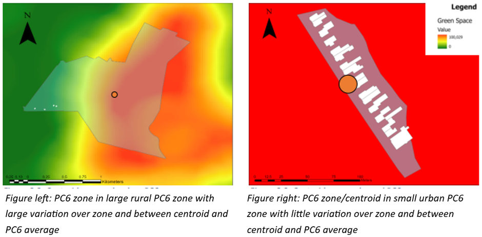
To illustrate this, I made the map example here below where you see that the zonal average in the indicated PC6 zone X of the mapped pollutant will be 18.4 µg/m³, while the extracted point concentration at PC6 centroid location X assigned to this PC6 zone will be 26.0 µg/m³.

The consequence is that in the case of the point centroid extraction, the house addresses get assigned a too high value, only representative to the point location close to the road.
On the other hand, in the case of the zonal average for the PC zone X, the value assigned will be an average of all grid cells (approximately 100 gridcells) within this PC6 zone. This might be in this example a more representative value, but fact is that the aggregation involves many gridcells where no houses are located.
As we are interested in the average pollution values at the address locations in the postal code zone it is a much better idea to go back to the pollution values extracted on the address level. These are the gridcell values corresponding to the house locations. In this way we take the average of the pollution values of all address locations falling in a certain postal code zone. In other words, we don’t need the GIS for this and can simply do a table aggregation (MEAN) with the PC6 code as the key field in SPSS. So, if the pollution values at the house locations A, B and C in the map above are respectively 16, 15 and 19 µg/m³, the average pollution concentration for PC6 area X will be 16.7 µg/m³, quite a bit lower than the values taken by zonal average or centroid point extraction from the GIS raster layer.
We expect that this ‘PC6 address aggregation approach’ results in much more accurate values for the rural areas where PC areas can be large and residence addresses can be unevenly distributed over the area. This is illustrated in the map examples below where you see a large variation in possible values within the PC6 zone in the figure on the left (and thus between centroid value and average PC6 value) and only a small variation in the urban setting in the figure on the right where you see only a minor variation in possible values within the PC6 zone in the figure on the left (and thus between centroid value and average PC6 value). In the PC6 zone in the rural area (left figure) you see as well 4 houses/address locations in the left part of the figure, these houses will have low variable values falling in the green range of the map legend and will not be well represented by the centroid value but also not by the average PC6 value. The average address value location using the this PC6 address aggregation approach will however give the most representative value for each of these houses.
November
2024
Summary:
Aggregation of noise data is now done with median values only.
Because of the logarithmic nature of the noise decibel scale the application of normal aggregation over space or time with average values would lead to large distortions to the real average noise level. This implies we should average over the inverse log of the logarithmic noise values. However, this is not possible in a standard GIS because of the huge sizes of the numbers involved. Solutions to this problem would require high amounts of processing power / time or mathematical work arounds. For these reasons we aggregate now only with median values.
Noise data that has been aggregated to PC6 and PC4 level prior to the Gecco project (2011 and earlier), still needs to be checked on the
aggregation method applied.
October 2024
Summary: For different years we now deliver the walkability score based on either 6 or 7 components, without or with the 7th public transport component.
From now on we deliver for the years 1989 up to 2012 the walkability score standard in 6 components and only for the years 2015 and 2017 we deliver the 7th component ‘public transport density’. This is because this 7th component is based on public transport data for 2018 which we consider too much subject to change over time and therefore unreliable for earlier years.
October
2024
Summary: The greenspace
component in the walkability score is now delivered as the standard urban green space component and/or as an extended green/bluespace component.
Our
definition of the greenspace component in the walkability score was up to now similar to the definition of urban green space commonly used in literature comprising the following land use classes
from the land use map series BBG - ‘Bestand BodemGebruik’:
· Parken en plantsoenen (parcs and public gardens)
· Bos (forest)
· Begraafplaats (graveyards)
· Day recreative areas
We offer now a more extended definition of the green (and blue) space component in which we also include agricultural vegetation (including pastures but excluding horticulture), dry and wet natural areas and all types of surface water. The reason for this extension is the increasing body of literature that refers to positive health effects not only of urban green space, but of all kind of green spaces, including agricultural green space such as grassland and meadows that are the dominant types of green space that surround Dutch cities (see Brauwbach et al. in WHO report 2021,) natural dry and wet spaces including surface water. To give some more literature examples regarding open green / public space and mental health:
-Francis et al (2012) demonstrate a positive relationship between open public space and mental health;
-Wood et al (2017) show that different types of public green space (not only nature, but also sport/ recreation) contribute to mental health;
-Alcock et al (2015) try to fill the research gap on the role of green space for mental health in more rural areas;
-Simoes et al (2022) show that there can be also a downside of living near agricultural areas when it concerns pesticide-treated farmland;
-Also White et al (2021) stress that the potential of other types of spaces apart urban green space associated with better mental health, such as blue spaces remains under-explored.
Moreover, the proximity and the view of different types of open green and blue spaces is also reflected into house prices / social value, see e.g. Luttik (2000), Cho et al (2008)
and Brander and Koetse (2011) who include agricultural green space at the urban fringe in their urban green space definition.
In the reference list below more references concerning the report between green-blue space and health, are included.
The only type of greenspace we consider as relevant greenspace but we did not (yet) included in the extended green-/bluespace definition are individual trees outside parcs and forest areas. In the maps below you can see that in some areas (here the dune area in the vicinity of Bloemendaal) individual trees can make up a significant part of green space but because of the scattered nature of trees is not represented as green space in the BBG land use maps.
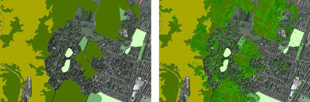
Green space land use classes without (left) and with individual tree crowns displayed on top (right)
January
2024
Summary: The high resolution greenspace density variable derived from the aerial photography (Infrared CIR file) based vegetation dataset from RIVM is now also available for the
year 2022.
The vegetation map for the year 2022 from RIVM derived among others from the aerial photography Infrared CIR file (0,25 meter resolution) is now also available on a resolution of 5x5 meter and 10x10 meter. The map on 5x5 meter resolution distinguishes between agricultural greenspace, Natura2000 vegetation, ‘Natuurnetwerk’ area and green space in other areas. It can however not distinguish between low vegetation, agriculture, trees and shrubs like the 2017 version of this map. The map on 10x10 meter resolution gives the percentage green per gridcel.
November
2023
Summary: The RIVM high resolution greenspace density variable is now improved by correcting low or zero greenspace values in gridcells corresponding to agricultural parcels that
were fallow during satellite data collection.
Our high resolution variable with greenspace density based on the RIVM 10 meter resolution vegetation maps for 2017 (all vegetation and low vegetation) has been corrected for seasonal effects / fallow in vegetation occurrence by the use of the dataset Basisregistratie Gewaspercelen (key register for arable plots - BRP ) for the corresponding year. Gridcells corresponding to parcels in the BRP have been assigned a vegetation coverage of 100%.
References
Alcock, I., White, M. P., Lovell, R., Higgins, S. L., Osborne, N. J., Husk, K., & Wheeler, B. W. (2015). What accounts for ‘England's green and pleasant land’? A panel data analysis of mental health and land cover types in rural England. Landscape and Urban Planning, 142, 38-46.
Brander, L. M., & Koetse, M. J. (2011). The value of urban open space: Meta-analyses of contingent valuation and hedonic pricing results. Journal of environmental management, 92(10), 2763-2773.
Braubach, M., Kendrovski, V., Jarosinska, D., Mudu, P., Andreucci, M. B., Beute, F., ... & Russo, A. (2021). Green and blue spaces and mental health: New evidence and perspectives for action.
Francis, J., Wood, L. J., Knuiman, M., & Giles-Corti, B. (2012). Quality or quantity? Exploring the relationship between Public Open Space attributes and mental health in Perth, Western Australia. Social science & medicine, 74(10), 1570-1577.
Li, H., Browning, M. H., Rigolon, A., Larson, L. R., Taff, D., Labib, S. M., ... & Kahn Jr, P. H. (2023). Beyond “bluespace” and “greenspace”: A narrative review of possible health benefits from exposure to other natural landscapes. Science of The Total Environment, 856, 159292.
Liu, D., Kwan, M. P., Kan, Z., & Wang, J. (2022). Toward a healthy urban living environment: Assessing 15-minute green-blue space accessibility. Sustainability, 14(24), 16914.
Luttik, J. (2000). The value of trees, water and open space as reflected by house prices in the Netherlands. Landscape and urban planning, 48(3-4), 161-167.
McDougall, C. W., Hanley, N., Quilliam, R. S., & Oliver, D. M. (2022). Blue space exposure, health and well-being: Does freshwater type matter? Landscape and Urban Planning, 224, 104446.
Pasanen, T. P., White, M. P., Wheeler, B. W., Garrett, J. K., & Elliott, L. R. (2019). Neighbourhood blue space, health and wellbeing: The mediating role of different types of physical activity. Environment international, 131, 105016.
Simoes, M., Huss, A., Janssen, N., & Vermeulen, R. (2022). Self-reported psychological distress and self-perceived health in residents living near pesticide-treated agricultural land: a cross-sectional study in The Netherlands. Occupational and environmental medicine, 79(2), 127-133.
Vert, C., Gascon, M., Ranzani, O., Márquez, S., Triguero-Mas, M., Carrasco-Turigas, G., ... & Nieuwenhuijsen, M. (2020). Physical and mental health effects of repeated short walks in a blue space environment: A randomised crossover study. Environmental Research, 188, 109812.
Völker, S., Heiler, A., Pollmann, T., Claßen, T., Hornberg, C., & Kistemann, T. (2018). Do perceived walking distance to and use of urban blue spaces affect self-reported physical and mental health? Urban forestry & urban greening, 29, 1-9.
White, M. P., Elliott, L. R., Grellier, J., Economou, T., Bell, S., Bratman, G. N., ... & Fleming, L. E. (2021). Associations between green/blue spaces and mental health across 18 countries. Scientific reports, 11(1), 8903.
Wood, L., Hooper, P., Foster, S., & Bull, F. (2017). Public green spaces and positive mental health–investigating the relationship between access, quantity and types of parks and mental wellbeing. Health & place, 48, 63-71.